Extracting lexicons from raw text automatically enables the creation of valuable linguistic resources that can serve multiple tasks. Depending on the method applied in extracting the lexicons, lexicons provide insights into the context of the text, they can be used in developing systems and applications as a source of contextual knowledge (e.g. question answering systems, text classification, translation…etc.), they can be used to find collocations, and they can help in creating taxonomies.
We will explore five lexicon extraction statistical methods in this article as the following:
- Simple frequency count.
- Pointwise Mutual Information (PMI).
- T-test.
- Chi-square test.
- Likelihood ratio.
Some parts from this article are depending on the content from the following paper:
Husain, F. & Uzuner, O. (2021). SalamREPO: an Arabic Offensive Language Knowledge Repository. Future Technologies and Innovations (FTI) Proceedings: 4th International Conference on Computer Applications & Information Security (ICCAIS’2021). March 19-21, Tunisia. https://fti-tn.net/iccais-2021-list-of-papers
Importing Dataset and Python Libraries
We download the full text of the holly Quran from Tanzil website. We select the format of the text to be simple clean without Tatweel and without signs of pause or sajda or rub-el-hizb to make it simpler for analysis. In addition, we choose the file format to be text (.txt).
Once you are done downloading the file to your device, you can upload it to the Colab project directory by selecting the icon on the left with an upward arrow to upload it to session storage. Then, choose the Quran text file you have on your device. The name of the file we are using is Quran-simple-clean.txt.
We start coding as usual by importing python libraries:
					# importing libraries
import numpy as np
import pandas as pd
import re
import nltk
nltk.download('stopwords')
from nltk.corpus import stopwords
import spacy
import string
import os
To read the Quran text file and print its content on the screen, use the following script:
					# reading the txt file
a_file = open("/content/quran-simple-clean.txt")

# print file content
lines = a_file.readlines()
for line in lines:
    print(line)

If you scroll down the output screen, you will notice that the file contains some English comment at the end that does not belong to the Quran content. It has some term-of-use conditions and version information, which are not relevant to our analysis. Thus, we will delete these lines using the following script:
					# delete last lines in the txt file that contains comments
# then save the quran text in another file called quran.txt

#with open("sample.txt", "r") as input:
with open("temp.txt", "w") as output:
    # iterate all lines from file
    for line in lines:
        # if line starts with symbol '#' then don't write it in temp file
        if not line.strip("\n").startswith('#'):
            output.write(line)

# replace temp file with quran.txt name file
os.replace('temp.txt', 'quran.txt')
Now, let’s print the content of the new quran.txt file to check if the comments are not there and to make sure that it only has Quranic text.
					b_file = open("/content/quran.txt")


b_lines = b_file.readlines()
for line in b_lines:
    print(line)

You can scroll down the output screen and check that it ends with the chapter/Sura “Surat Al Naas”. Thus, all text in the file is from the Quran text.
I prefer to convert the txt file to a dataframe and then start analysis as that can help to add columns for each preprocessing step performed on the text, which can support comparison among the different versions of the text used based on the analysis procedures performed.
					# convert txt file to dataframe
data = pd.read_csv('quran.txt', sep=',', header = None)
data

To process the text easily using an array, we extract the Quranic text into an array as the following:
					# selecting the input array from the dataframe to process
raw_data = data.iloc[:,0]
raw_data

We use the NLTK library to tokenize the text. We need to split the text based on the words/string, which can support the extraction of lexicons. We save the tokenized text into a new column “tokens” in the same dataframe table that we created before. The full dataframe is shown below under the script to check differences between the raw text and the tokenized text.
					# import library
import nltk
nltk.download('punkt')

# tokenize text and saving the output to a new column "tokens"
data['tokens'] = raw_data.apply(lambda x: nltk.word_tokenize(x))

# print the entire dataframe including the tokenized text
data

All tokens were merged into one list to prepare the text for lexicon extraction as the following:
					#turn all tokens into one single list

list_tokens = [item for items in data['tokens'] for item in items]

# check tokens list
list_tokens

Lexicons Extraction Methods
1. Simple Frequency Count of Adjacent Words
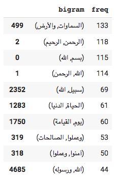
This method is very simple. It depends on the word order by their frequencies in text. The main issues that usually occur in its output is that it is too sensitive to very frequent pairs, which might represent pronouns, articles, and prepositions that are not valuable to the context of the text.
In all examples below, we will apply the lexicon extraction methods for two length: bigrams for two words lexicons and trigrams for three words lexicons. Initialize NLTK’s library function for Bigrams and Trigrams Finder as the following:
					# intialize bigrams and trigrams measures and extract them from the text
bigrams = nltk.collocations.BigramAssocMeasures()
trigrams = nltk.collocations.TrigramAssocMeasures()

bigramFinder = nltk.collocations.BigramCollocationFinder.from_words(list_tokens)
trigramFinder = nltk.collocations.TrigramCollocationFinder.from_words(list_tokens)

# create frequency table
bigram_freq = bigramFinder.ngram_fd.items()
bigramFreqTable = pd.DataFrame(list(bigram_freq), columns=['bigram','freq']).sort_values(by='freq', ascending=False)

# print table head
bigramFreqTable.head().reset_index(drop=True)

					# print most frequent top 15 bigrams
bigramFreqTable[:15]

You might notice that most of the top frequent frequency bigrams include particles and pronouns, which are called stop words in Natural Language Processing (NLP). For more detail about the meaning of stop words, please refer to our previous blog.
The following method remove stop words from the text.
					#function to remove stop words
def rightTypes(ngram):
    #if stop word:
        #return False
    ar_stopwords = set(stopwords.words('arabic'))
    for word in ngram:
        if (word in ar_stopwords):
            return False
    sentence = ngram
    return True
Applying the filtering method to the frequency based bigrams and printing the top 50 filtered bigrams.
					#filter bigrams
filtered_bi = bigramFreqTable[bigramFreqTable.bigram.map(lambda x: rightTypes(x))]

# print top 50 filtered bigrams
filtered_bi[:50]

					# extracting trigrams and save the results into a table
trigram_freq = trigramFinder.ngram_fd.items()
trigramFreqTable = pd.DataFrame(list(trigram_freq), columns=['trigram','freq']).sort_values(by='freq', ascending=False)

# checking the head of the table
trigramFreqTable.head().reset_index(drop=True)

					# printing the top 50 frequency based trigrams
trigramFreqTable[:50]

					# filtering the content
filtered_tri = trigramFreqTable[trigramFreqTable.trigram.map(lambda x: rightTypes(x))]

#print the top 50 filtered frequency based trigrams
filtered_tri[:50]

At the end of the article, we will save all output to a CSV file to be downloaded for further analysis. Thus, in the following script, we save all outputs into arrays as the following:
					# saving the resulted bigrams and trigrams into arrays to organize the overall output later
freq_bi = filtered_bi[:50].bigram.values
print(freq_bi)
freq_tri = filtered_tri[:50].trigram.values
print(freq_tri)

# saving the resulted frequencies into arrays to organize the overall output later
freq_bi_no = filtered_bi[:50].freq.values
print(freq_bi_no)
freq_tri_no = filtered_tri[:50].freq.values
print(freq_tri_no)
“Indeed, in the creation of the heavens and earth, and the alternation of the night and the day, and the [great] ships which sail through the sea with that which benefits people, and what Allah has sent down from the heavens of rain, giving life thereby to the earth after its lifelessness and dispersing therein every [kind of] moving creature, and [His] directing of the winds and the clouds controlled between the heaven and the earth are signs for a people who use reason.”
Sūrat l-baqarah [Quran 2:164]
2. Pointwise Mutual Information (PMI)
The main concept of Pointwise Mutual Information (PMI) is borrowed from the information theory. The PMI measures how much more the two or three words co-occur than if they were independent.
To extract bigrams based on the PMI method, we use the NLTK library as it provides modules for most lexicon extraction methods. The following script is used:
					# extract bigrams based on PMI and create a table
bigramFinder.apply_freq_filter(50)
bigramPMITable = pd.DataFrame(list(bigramFinder.score_ngrams(bigrams.pmi)), columns=['bigram','PMI']).sort_values(by='PMI', ascending=False)
print (bigramPMITable)

Looking to the output above, you might notice multiple stop word, such as من/from, في/in, كانوا/were …etc. Thus, applying the filtering method as the following script shows to remove stop words is very important.
					# filtering the PMI bigrams and printing the top 50
filtered_biPMI = bigramPMITable[bigramPMITable.bigram.map(lambda x: rightTypes(x))]
filtered_biPMI[:50]

We also extract trigrams as we did using the other previously discussed methods. The following script extract the trigrams and organize them into a dataframe table, then printing the top trigrams:
					# extracting the trigrams, saving them into a dataframe table, and printing the top 50
trigramFinder.apply_freq_filter(50)
trigramPMITable = pd.DataFrame(list(trigramFinder.score_ngrams(trigrams.pmi)), columns=['trigram','PMI']).sort_values(by='PMI', ascending=False)
trigramPMITable[:50]

To remove stop words from the output, we also apply the filtering method defined before as the following:
					# filtering the output to remove stop words and printing the top 50
filtered_triPMI = trigramPMITable[trigramPMITable.trigram.map(lambda x: rightTypesTri(x))]
filtered_triPMI[:50]

As we did before, all results are saved to arrays as the following:
					# saving the resulted bigrams and trigrams into arrays to organize the overall output later
pmi_bi = filtered_biPMI[:50].bigram.values
pmi_tri = filtered_triPMI[:50].trigram.values

# saving the resulted frequencies into arrays to organize the overall output later
pmi_bi_no = filtered_biPMI[:50].PMI.values
pmi_tri_no = filtered_triPMI[:50].PMI.values

3. T-test
The t-test takes a sample from the data and assumes that the sample is drawn from a normal distribution with the same mean (𝜇).In the following script, we apply the method student_t from the NLTK library to extract bigrams, then we create a dataframe table and print the top results:
					# bigrams extraction and creating table
bigramTtable = pd.DataFrame(list(bigramFinder.score_ngrams(bigrams.student_t)), columns=['bigram','t']).sort_values(by='t', ascending=False)
bigramTtable.head()

We apply the filtering method we defined before to remove stop words from the output. The following script shows how we apply the filtering method. We also print the top 50 bigram results to check the output as the following:
					# filtering the bigrams
filteredT_bi = bigramTtable[bigramTtable.bigram.map(lambda x: rightTypes(x))]
filteredT_bi[:50]

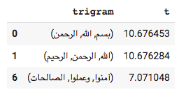
As we did earlier, trigrams are extracted for the t-test as well as the following:
					# extracting trigrams
trigramTtable = pd.DataFrame(list(trigramFinder.score_ngrams(trigrams.student_t)), columns=['trigram','t']).sort_values(by='t', ascending=False)
trigramTtable.head()

We filtered the trigram output list to remove any stop words as the following:
					# filtering trigrams list
filteredT_tri = trigramTtable[trigramTtable.trigram.map(lambda x: rightTypes(x))]
filteredT_tri.head(50)

To add the results to the overall result CSV file at the end, we create arrays for the results as the following:
					# saving the resulted bigrams and trigrams into arrays to organize the overall output later
t_bi = filteredT_bi[:50].bigram.values
t_tri = filteredT_tri[:50].trigram.values

# saving the resulted frequencies into arrays to organize the overall output later
t_bi_no = filteredT_bi[:50].t.values
t_tri_no = filteredT_tri[:50].t.values
4. Chi-Sqaure
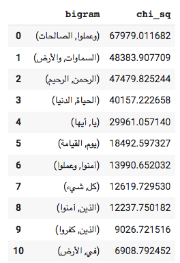
The chi-square test (𝑥2) assumes that the sample is not normally distributed. It compares observed frequencies to expected frequencies. The larger the difference, the larger the confidence that the co-occurred words are not co-occur by chance.
We apply the chi_sq from the NLTK library to find the bigrams and trigrams based on the chi-square test as the following script shows:
					# extracting bigrams and organizing them into a table
bigramChiTable = pd.DataFrame(list(bigramFinder.score_ngrams(bigrams.chi_sq)), columns=['bigram','chi_sq']).sort_values(by='chi_sq', ascending=False)
bigramChiTable.head(50)

As earlier, the output list should get filtered as the following:
					# Filtering the output to remove stop words
filtered_biChi = bigramChiTable[bigramChiTable.bigram.map(lambda x: rightTypes(x))]
filtered_biChi[:50]

Now, we will extract the trigrams , save them to a dataframe table, and filtered them to remove stop words as the followings:
					# extracting trigrams and saving result to a dataframe table
trigramChiTable = pd.DataFrame(list(trigramFinder.score_ngrams(trigrams.chi_sq)), columns=['trigram','chi_sq']).sort_values(by='chi_sq', ascending=False)
trigramChiTable.head(50)

					# filtering trigram output
filtered_triChi = trigramChiTable[trigramChiTable.trigram.map(lambda x: rightTypes(x))]
filtered_triChi[:50]

To save the overall results in one result CSV file, we create arrays for the output as the following:
					# saving output to arrays to be used at the end of the project
chi_bi = filtered_biChi[:50].bigram.values
chi_tri = filtered_triChi[:50].trigram.values

chi_bi_no = filtered_biChi[:50].chi_sq.values
chi_tri_no = filtered_triChi[:50].chi_sq.values
5. Likelihood Ratio
The Likelihood ratio is more appropriate for sparse data than the previous approaches. It is a number that tells us how much more likely one word in the bigram/trigram is depending on the other word.
We apply the NLTK function “Likelihood_ratio” to extract bigrams and trigrams based on the Likelihood ratio. The following script shows how it is applied:
					# extracting bigrams to a dataframe table
bigramLikTable = pd.DataFrame(list(bigramFinder.score_ngrams(bigrams.likelihood_ratio)), columns=['bigram','likelihood_ratio']).sort_values(by='likelihood_ratio', ascending=False)
bigramLikTable.head()

We then apply the filtering function defined before to remove stop words as the following:
					# filtering the trigram list
filteredLik_bi = bigramLikTable[bigramLikTable.bigram.map(lambda x: rightTypes(x))]
filteredLik_bi.head(50)

Similar to the previous methods, we also extract trigrams and filtered them as the following:
					# extracting trigram
trigramLikTable = pd.DataFrame(list(trigramFinder.score_ngrams(trigrams.likelihood_ratio)), columns=['trigram','likelihood_ratio']).sort_values(by='likelihood_ratio', ascending=False)
trigramLikTable.head()

					# filtering the trigram list
filteredLik_tri = trigramLikTable[trigramLikTable.trigram.map(lambda x: rightTypes(x))]
filteredLik_tri.head(50)

Arrays are created to save the results and to create a large CSV file that contains all methods’ outputs.
					# creating arrays to save the results
lik_bi = filteredLik_bi[:50].bigram.values
lik_tri = filteredLik_tri[:50].trigram.values

lik_bi_no = filteredLik_bi[:50].likelihood_ratio.values
lik_tri_no = filteredLik_tri[:50].likelihood_ratio.values
Creating Comparison Tables
The Bigrams Table
Having the results from all methods next to each other in one large table supports better comparison to find patterns among them. Thus, we aggregate all results to one large dataframe table and convert it to a CSV file to be downloaded and saved for further analysis as the following:
					# aggregate results from all methods of the bigram extraction to one table
bigramsCompare = pd.DataFrame([freq_bi, freq_bi_no, pmi_bi, pmi_bi_no, t_bi, t_bi_no, chi_bi, chi_bi_no, lik_bi, lik_bi_no]).T
bigramsCompare.columns = ['Frequency', 'Freq.','PMI', '%','T-test', '%','Chi-Sq Test', '%','Likeihood Ratio Test', '%']

# saving the resulted table to a csv file
bigramsCompare.to_csv('bigramsCompare.csv', sep=',', index=False,encoding='utf-8-sig')
The Trigram Table
As we just did for the bigram results, we also follow the same steps for the trigram outputs.
					#aggregate results from all methods of the trigram extraction to one table
trigramsCompare = pd.DataFrame([freq_tri, freq_tri_no, pmi_tri, pmi_tri_no, t_tri, t_tri_no,  chi_tri,chi_tri_no, lik_tri, lik_tri_no]).T
trigramsCompare.columns = ['Frequency', 'Freq.','PMI', '%','T-test', '%','Chi-Sq Test', '%','Likeihood Ratio Test', '%']

# saving the resulted table to a csv file
trigramsCompare.to_csv('trigramsCompare.csv', sep=',', index=False,encoding='utf-8-sig')

In this article, we review some examples of lexicon extraction methods. We recommend to increase the accuracy of the output by adding some filtering techniques based on Part-of-Speech tagging tools to provide specific patterns in the extracted lexicons. The concept of “Collocation” is also very similar to our topic, we suggest this draft chapter from Stanford NLP group to learn about the available tools and methods in extracting terms.
The entire code used in this exercise is available on this Github repository and on this Colab Project. We hope you find this article useful and informative. Please let us know if you have any question or comment by commenting on this article or by email.
Citation
For attribution in academic contexts, please cite this work as:
Husain F., “Extracting Quranic Lexicons”, The Information Science Lab, 2 December 2022.
Note: All photos presented in this article are captured by the author at the Arabic Islamic Science Museum in Sheikh Abdullah Al Salem Cultural Centre in Kuwait.


